Description of DQN

DQN is an algorithm where a Q learning framework with a neural network proceeds as a nonlinear approximation on a state-value function. Unlike original Q-learning that requires a great amount of time to create a Q-table and memory to save history, which thus has its limitations in a large-scale problem, this novel algorithm has 2 main advantages to overcome these problems, i.e., experience replay and target network.

With replay buffer, DQN stores the history for off-policy learning and extracts samples from the memory randomly. Because in reinforcement learning, the observed data are ordered. Ordered data is prone to overfitting current episodes. So DQN uses experience replay to solve this problem. Experience replay stores all necessary data (state transitions, rewards and actions) for performing Q learning and extracts sample data from the memory randomly to update. It reduces correlation between data.

In addition, DQN is optimized on a target network with fixed parameters updated periodically so that the Q-network is not changed frequently and makes training more stable.

Configurations

In our experiments, we mainly tune the following parameters for comparison.

Memory Size: Maximum size of the replay memory.
lr: Learning rate, used for optimizer.
γ: Discount factor.
Using Win Memory: Whether we use another replay buffer, which will explain on section 3.3.
Decay: Epsilon decay rate
Average Reward: Evaluate the final model 10 times and average the rewards.

CartPole

All the experiments are implemented in Google Colab. The parameters areexplained as follows. 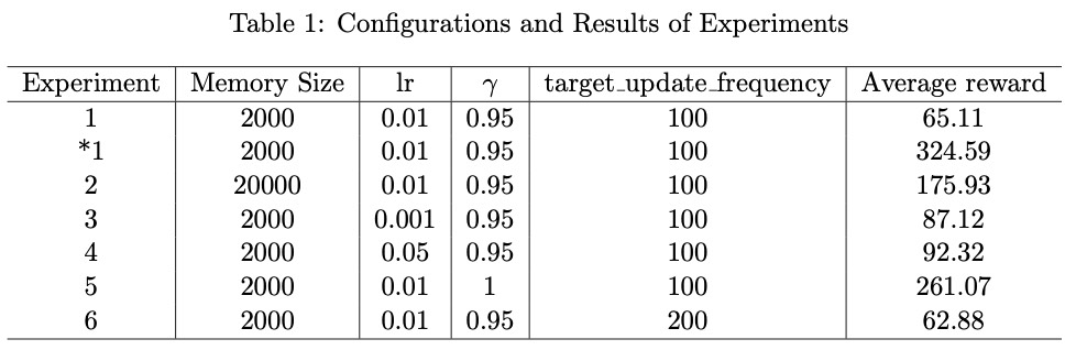Note that the prefix “*” for is a distinguished result from the first Experiment 1.

Discussion

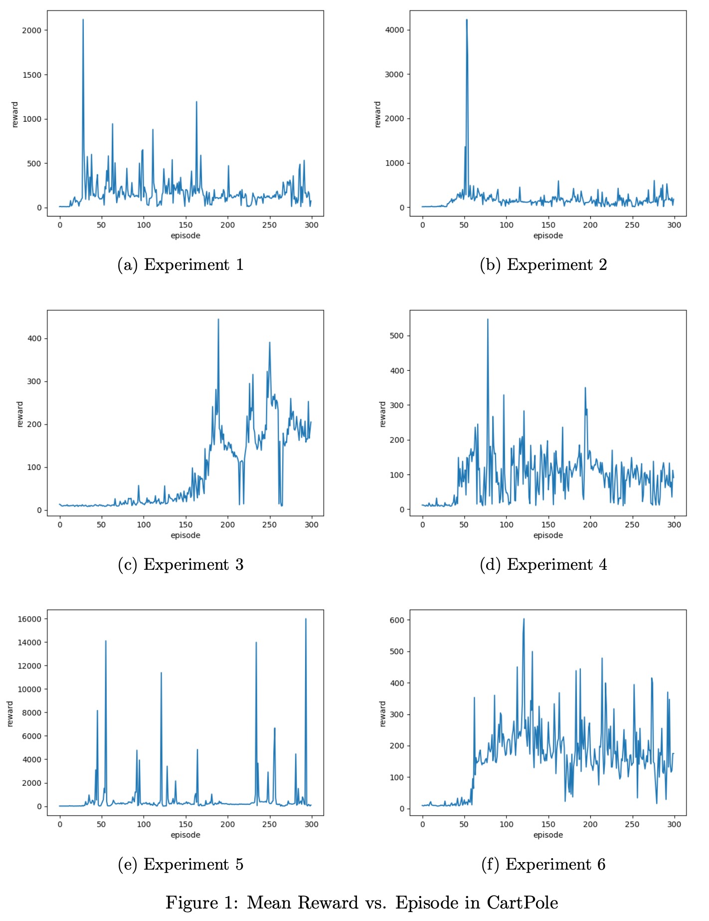
From Figure 1, it can be found that all figures show messy patterns for rewards. Experiment 1 is selected as a baseline for comparison. In Experiment 2, the memory size is larger and the averaged reward is more satisfactory. With more memory, the model tends to select different samples for gradient descent, so that the result will be more robust. Experiment 3 and 4 use different learning rates. Theoretically, a smaller learning rate gives a smooth and slowly-growing curve, and the larger one produces a more curve with violate fluctuation. However, Figure 1c and 1d show little relationship with expected tendency. Experiment 5 chooses a larger gamma that enables the current state to have a more impact on the future state and thus larger gamma leads to a larger reward, which is in line with our result. In experiment 6, we do not notice any distinguished differences caused by train update frequency, which may have to be set on a larger scale to generate a distinction. Anyway, it seems that there are no obvious differences and similarities among figures, and it is difficult for us to summary the regulations.

Reward Function

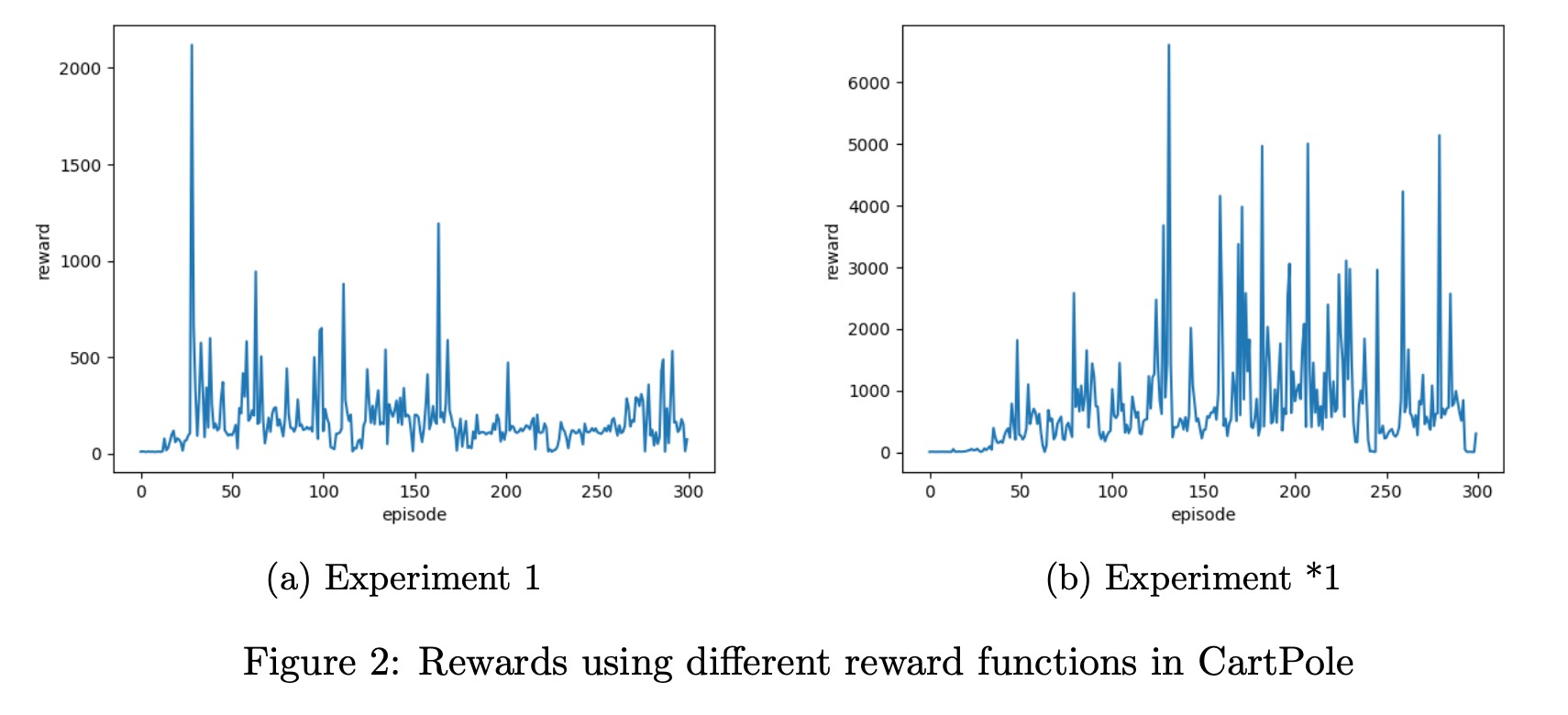As you can see in experiment 1 and *1, the hyperparameters are the same but with different reward functions. In experiment 1, the reward function is simple, the agent gets reward 1 when the game was not done, otherwise, the reward is -1. But in experiment *1, we changed the reward function which is based on the state. When the car is closer to the midpoint, the reward is higher. When the angle between the flag and the horizontal line is closer to 90 degrees, the reward is higher, and vice versa. The results revealed that a good reward function can make a huge difference in performance when it comes to Reinforcement Learning, which can speed up the process of agent learning.

Results of Pong

All the experiments are implemented in Google Colab with 2.5 million frames. The parameters are explained as follows.

Discussion

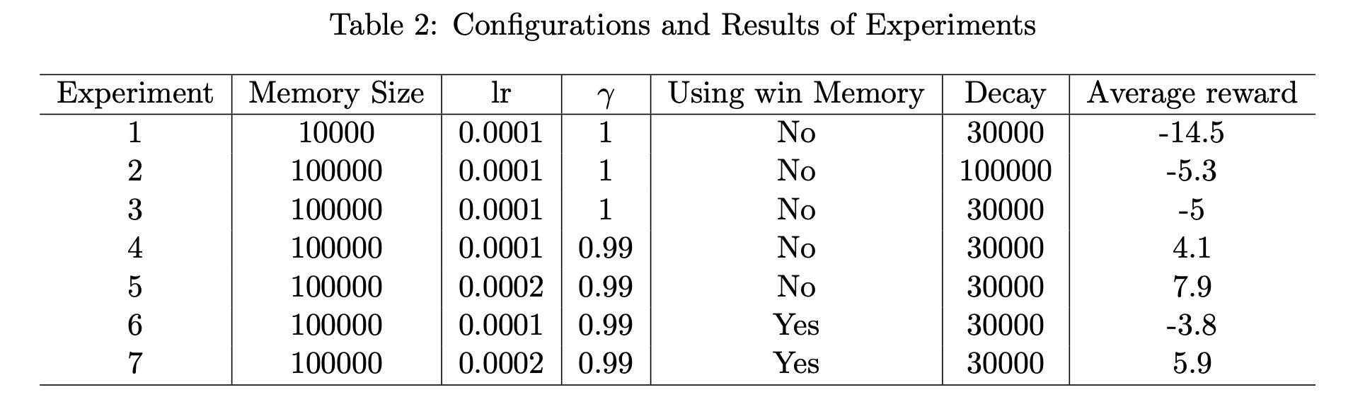
The curve in the resulting figures may not be a good description of the performance of the current model, because we take the average of the most recent 10 episodes as the score of the current model. So when the experiment is over, we re-evaluated the average value ten times with the saved model. This result will be more representative. We implement multiple experiments based on the environment Pong-v0. In general, the results are basically satisfactory. The configuration of the model and its performance(Column Average reward) are displayed as Table 2.

Replay Memory Size

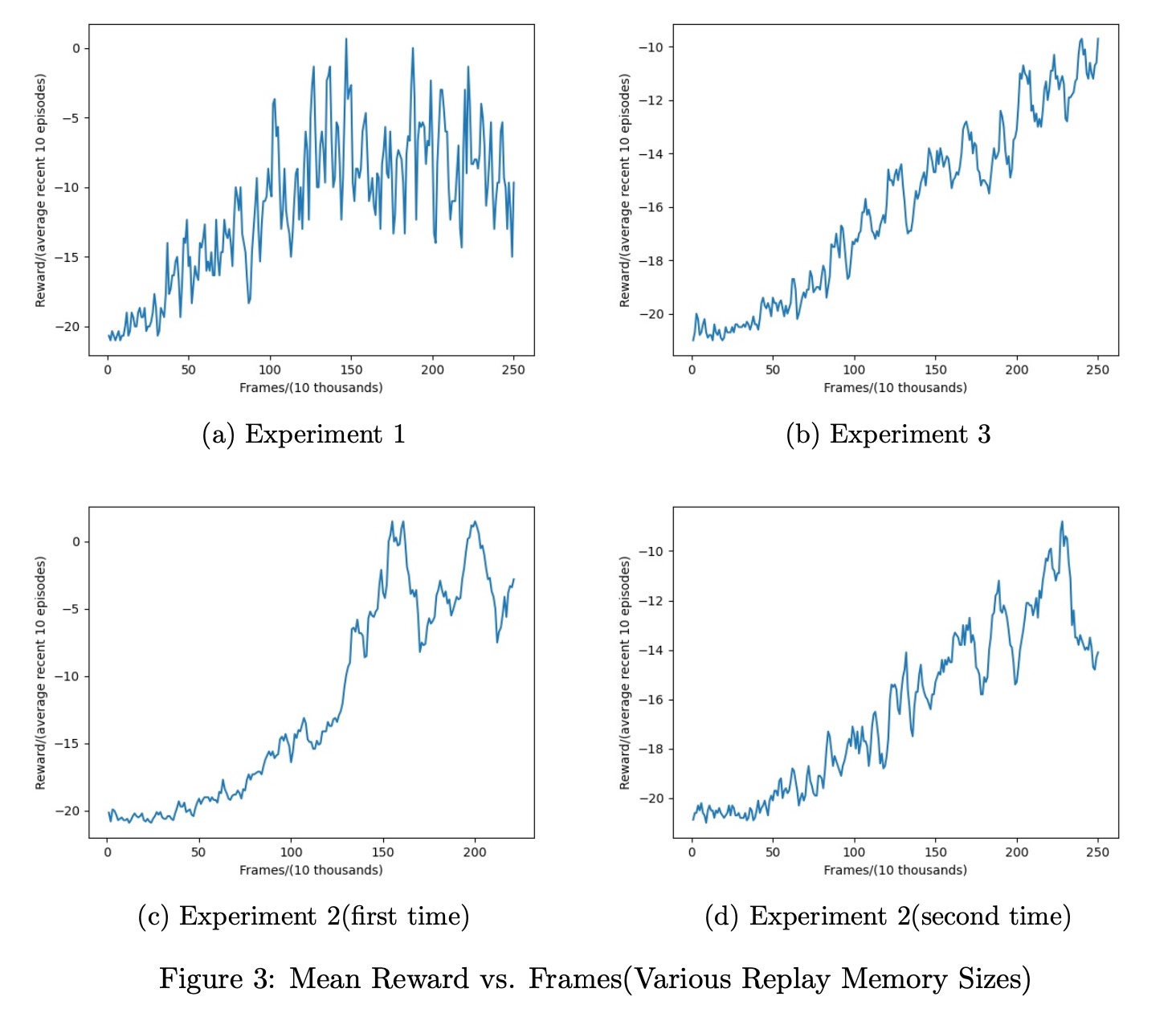
Figure 3 visualizes the results of Experiment 1, 2 and 3. It can be observed from 3a that when the replay memory size is 10000, the performance of the model is unstable, comparing with the averaged reward trend in Experiment 3. The reason for the differences is that the larger the experience replay, the less likely you will sample correlated elements, hence the more stable the training of the NN will be. However, a large experience replay requires a lot of memory so the training process is slower. Therefore, there is a trade-off between training stability (of the NN) and memory requirements. In these three experiments, the gamma valued 1, so the model is unbiased but with high variance, and also we have done the Experiment 2 twice, second time is basically satisfactory (as you can see in the graph), but first Experiment 2 were really poor which is almost same with Experiment 3. The result varies a lot among these two experiment due to the gamma equals to 1.

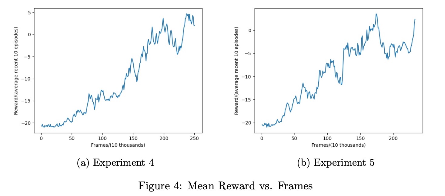
Learning Rate

Now we discuss how learning rate affects the averaged reward. It is found from Figure 4 that a high learning rate has relatively large volatility on the overall curve, and the learning ability is not stable enough, but the learning ability will be stronger.

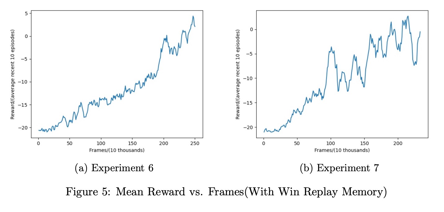
Win Replay Memory

Here we try a new way to train our model and create a win replay memory for those frames that our agent gets reward 1. After 0.4 million frames, we start to randomly pick 5 samples from this win memory and then train the model every 5 thousand frames. The idea is for this kind of memory, the loss may vary a lot, so the model will tune the parameters more. But the results show that the performance is basically the same or even worse than that of learning rate = 0.0002.

Summary

Each experiment takes 4h on Google Colab. We achieve 10-time average reward of 7.9 as the best result that is better than Experiment 1(suggested configuration on Studium), although the result is somewhat random and may be unreproducible. It seems that the models with higher learning rate(0.002) perform better, but its reward influtuates more sharply.

Github

If you want to know more details of our works, please check our reports in Github.