Language Model
word2vec
Word2Vec is a popular algorithm used in Natural Language Processing (NLP) for generating word embeddings. We need Word2Vec for several reasons:
-
Word representation: Word2Vec allows us to represent words as dense vectors in a continuous vector space. This representation captures semantic and syntactic relationships between words, enabling machines to better understand and process natural language.
-
Feature extraction: Word2Vec captures meaningful linguistic features from the input text, such as word similarities and contextual relationships. These features can be used as input for various downstream NLP tasks like sentiment analysis, text classification, machine translation, and named entity recognition, improving their performance.
-
Dimensionality reduction: Word2Vec reduces the high-dimensional space of words into a lower-dimensional space while preserving semantic relationships. This reduction makes the computations more efficient and manageable, especially when dealing with large amounts of text data.
-
Contextual understanding: Word2Vec models, such as Skip-gram and Continuous Bag of Words (CBOW), consider the surrounding words or context of a target word when learning word embeddings. This contextual understanding enables the model to capture word meanings based on their surrounding words and improve the accuracy of semantic relationships.
Overall, Word2Vec plays a crucial role in various NLP applications by providing efficient word representations, feature extraction capabilities, and improved contextual understanding.
word2vec models
The common word2vec models are Skip-gram and Continuous Bag of Words(CBOW), consider the surrounding words or context of a target word when learning word embeddings. Both models have two curcial parameters, context word and center word vectors.
CBOW
This method takes the context of each word as the input and tries to predict the word corresponding to the context.
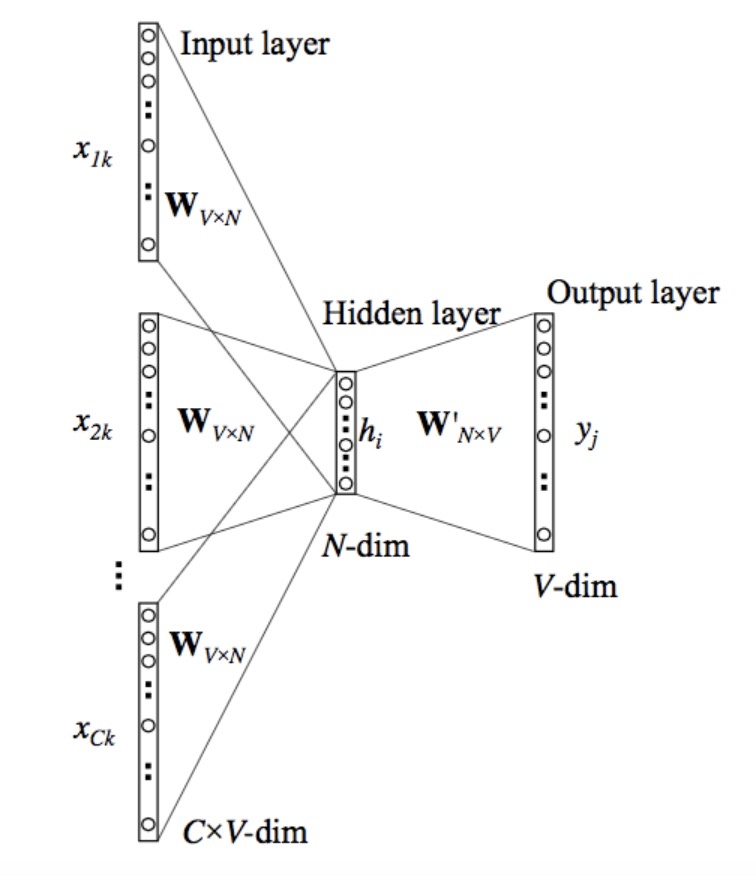 The above model takes C context words. When $Wvn$ is used to calculate hidden layer inputs, we take an average over all these C context word inputs.
The input or the context word is a one hot encoded vector of size V. The hidden layer contains N neurons and the output is again a V length vector with the elements being the softmax values. Let’s get the terms in the picture right:
- $Wvn$ is the weight matrix that maps the input x to the hidden layer (VN dimensional matrix) -$W’nv$ is the weight matrix that maps the hidden layer outputs to the final output layer (NV dimensional matrix)
Skip-gram
This method takes the center words as the input and tries to predict the word corresponding to the center.
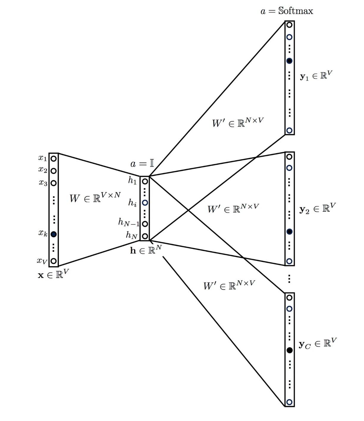 The above model takes a center word as input and outputs C probability distributions of V probabilities, one for each context word.
The more information related to Hierarchical Softmax and Skip-Gram Negative Sampling can be found here.
seq2seq
Recurrent Neural Networks
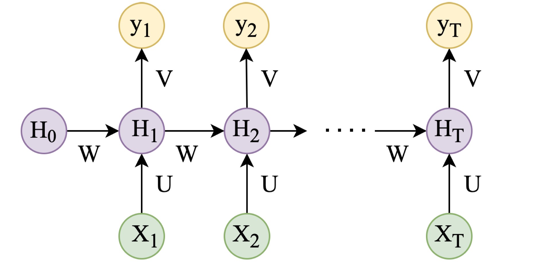 The design of RNN solves the continuous input space, such as time continuous and space continuous input. Another difference with feed-forward neural networks is that the output format is also a sequence. Given a sequence of input $X = (X_1,X_2,…,X_T)$, and the standard RNN derives a sequence of outputs $y = (y_1, y_2, …, y_T)$ by the following equations and a more intuitive structure displayed above.
Herein, units H, X, and y represent the hidden, input, and output units, respectively. The parameter W, U, and V are the weights that need to be learned by iterating the loss and backpropagation. The RNN structure is suitable for solving the input with any length since the parameters are predominated by W, U, and V . RNN maintains an activation function for each layer, making the model extremely deep when the input space is enormous. Extremely deep models lead to a series of problems, such as vanishing or exploding gradients, which makes the training of RNN difficult.
Long Short-Term Memory
The central novel concept of LSTM architecture is the introduction of manipulated gates and short-term memory. These two concepts are excellent solutions to the difficulty of RNN in learning time dependencies beyond a few time steps long. The presence of the LSTM structure successfully solved the problem of gradient vanishing that appears during the training of the vanilla RNN.
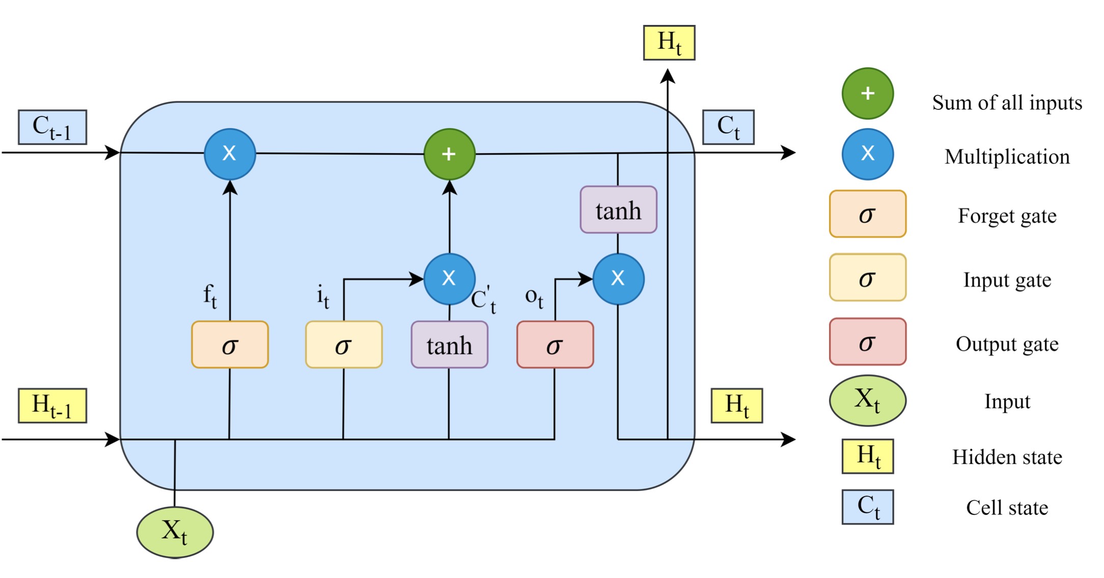
Forget gate
The introduction of forget gates allows the LSTM to reset its state, remember common behavioral patterns, and forget unique behaviors, improving the model’s generality and ability to learn sequential tasks. The information from the previously hidden unit $H_{t-1}$ and current input $X_t$ are passed through the forget gate ($f_t$) and will be rescaled to 0 to 1. The value closer to 0 means forget, and approaching one means to keep. The computation formula is presented below (W and b represent weights and bias, respectively).
\[f_t = \sigma(W_f(H_{t-1}, X_t) + b_f)\]Input gate
The design of the input gate is used to update the cell state. The input gate decides which values of $H_{t-1}$ and $X_t$ need to be updated for computing the new cell state $C_t$. The hidden state $H_{t-1}$ and input $X_t$ information are passed into the tanh function and rescaled between -1 and 1 to help regulate the model. Then we multiply the outputs from the sigmoid and the tanh functions. The output of the sigmoid function decides which information is essential to keep from the tanh output. The new cell state is the summation of the forget and input gate. The following equations describe the whole process.
\[i_t = \sigma(W_i(H_{t-1}, X_t) + b_i)\] \[C^{'}_t = tanh(W_c(H_{t-1}, X_t) + b_c)\] \[C_t = f_t C_{t-1} + i_t C^{'}_t\]Output gate
The output gate determines the value of the following hidden state $H_t$, and $H_t$ contains the value of the previous input, so the value of $H_t$ can also be used to predict. The previous information $H_{t-1}$ and current input $X_t$ are passed into a sigmoid function, and then the updated cell state C is squeezed by the tanh function between -1 to 1. Then we multiply the output from the tanh and the sigmoid, and the outcome is $H_t$, then $C_t$ and $H_t$ move to the next time step. The corresponding formulas are as follows.
\[o_t = \sigma(W_o(H_{t-1}, X_t) + b_o)\] \[H_t = o_t tanh(C_t)\]Transformers
The Transformers model is a powerful and popular approach in the field of natural language processing (NLP). At the core of the Transformers model lies the self-attention mechanism, which enables the model to handle dependencies between different positions in the input sequence simultaneously. This capability makes Transformers highly effective in processing long text sequences and modeling semantic relationships.
Firstly, the inputs will be transfer to input embedding, then add positional encoding as input of encode part. The encode part consist of two layer Multi-Head Attention and Feed Forward, and both with residual connection. Multi-head learns more aspects of inputs, and multi-layer makes each layer learn different level attention representation. Decode module almost have the same structure except the masked attetion, since the model is not supposed to see the full outputs.
![]()
One of the most renowned Transformer models is BERT (Bidirectional Encoder Representations from Transformers), which is a pre-trained language model used for various NLP tasks such as text classification, named entity recognition, sentiment analysis, and more. BERT achieved breakthrough results in natural language understanding tasks and has been widely adopted both in industry and academic research.